Overview
As Wayfair technology teams begin their replatforming journeys, more engineers will make decisions for their single purpose database. Choosing the right database technology is one of the most important decisions you can make when building a new microservice. If you realize down the line that you have made the wrong choice, migrating to another database can be a costly and risky procedure. We committed to Google as our cloud platform provider, and they offer multiple robust database options. Learning enough about all of them to make an informed decision can be a steep hill to climb; therefore, we set out to streamline this process, and provide our teams with a guide to help make these decisions.
For the purposes of this guide, we chose to analyze five of GCP’s database technologies:
Creating the Guide
General Approach
We can sum up a general approach to making a database decision in a few simple steps:
- Work with your product team to gather your functional and non-functional requirements both for now and 3-5 years out.Note: speed of development can be a non-functional requirement.
- Find all the datastores that meet your requirements.
- Pick the cheapest one.
Sounds easy enough, but first we needed to identify some categories of criteria that teams could use to help identify and evaluate their requirements.
Evaluation Criteria
Next, we identified some criteria for decision making. Having a basic understanding of application needs for these categories will help decision making and eliminate options that do not satisfy the requirements.
It’s important that we make the distinction here between “decisive criteria” and “considerations.” For example, cost is a consideration (something to be aware of but unlikely to drive the decision), whereas availability is a decisive criterion.
Decisive Criteria
When choosing a database, teams will have certain requirements that must be met. These are the “decisive criteria” and they are the most important to evaluate for the team’s specific application needs. Some types of Decisive Criteria include:
- Availability: Define SLOs for how much downtime the service is allowed.
Data Consistency: Refers to having a consistent view of data. For the purposes of this guide, we divide his into three categories:
- Strong trans regional consistency means that information should be immediately available to be read in all regions (this is what Spanner is known for).
- Strong regional consistency with eventual trans regional consistency means that data written in a particular region will be immediately available to be read in that region, and eventually will be available to be read from other regions.
- True eventual consistency means that there may be some lag between when the data is written and when it can be read, regardless of region.
Data Structure: This can be a bit more fluid and could be considered a consideration instead:
- Structured data is data that fits a standardized format, with a well-defined structure. This type of data fits well in a relational model.
- Unstructured data does not conform to a particular model and has no easily identifiable structure.
How complex are your query patterns?
- Analytics?
- Do you just need retrieval by key, or also by various other parameters?
- Do you also need fuzzy search on the data?
- Location: Where are you receiving traffic from? (e.g., US only, globally, single region)
Performance
Latency: The time cost incurred by a given database operation. Some applications can tolerate more latency than others. Keep in mind that consistency goes hand in hand with latency considerations. If a service occasionally needs strong consistency, some DB technologies will allow you to trade off latency for this by reading from/writing to the master region (Bigtable, Spanner). Some questions to ask include:
- How often are there writes?
- Can a caching strategy give the service the overall latency it needs?
Scalability
- The need for a massive scale and millions of writes per second will rule out less performant choices.
- The database's ability to scale along with the application will help narrow the search. For example, Cloud SQL can only scale vertically (for writes), whereas BigQuery, Bigtable, Firestore and Spanner can all scale horizontally.
Considerations
When choosing a database, it is important to consider certain additional criteria for the specific needs of the application (these are things that are important to be aware of, but in most cases are unlikely to be a deciding factor):
Cost: always a concern when choosing infrastructure. Teams should aim to choose solutions with the lowest cost possible. They should be aware of the cost structures for the various choices:
Ease of development
- Ease of developing database interfaces
- Local development - it is worth at least considering how easy it is to set up containers for local development for the various options (for example, a local emulator for BigQuery does not exist)
- Ease of modifying the database schema
- “Easy Button”: Wayfair provides workflows for provisioning certain database infrastructure, saving teams time and effort.
- SOX: What degree of effort is involved with establishing SOX compliance for a given database option?
Gathering Latency Data
In order to be able to make the best recommendation between the various database choices, we also needed latency data. As mentioned above, latency is the time cost incurred by a given database operation. Google publishes information on throughput and scaling, but they do not publish latency metrics. So, we set out to gather them ourselves.
This is not the first time that we have conducted such a test. See this article on Quantifying Google Cloud Spanner’s Geographic Latency for a very detailed writeup on a previous benchmarking exercise.
For the purposes of our guide, we decided to test our five DB options using several different configurations with different regions:
BigQuery
- Multi Region (US)
Bigtable
- Single region (us-central1)
- Multi Region (US) - clusters in us-central1, us-east4, us-west1
- Multi Region (EU) - clusters in europe-west3, europe-west4
- Global - clusters in us-central1, us-east4, us-west1, europe-west3, europe-west4
Cloud Spanner
- Single region (us-central1)
- Multi Region (US) - nam12
- Multi Region (EU) - eur6
- Three continent (nam-eur-asia1)
Cloud SQL
- Single region (us-central1)
Firestore (no single region or global configuration options available)
- Multi Region (US)
- Multi Region (EU)
The Application
We needed an application or script to gather the metrics. We decided to use a stripped down Basket microservice and chose Spring Boot for our application framework. The service would integrate with all five database options and provide a simple GraphQL API for testing. It would run in GKE clusters in the five different GCP regions we were interested in (us-central1, us-east4, us-west1, europe-west3, and europe-west4) and provide metrics to Google’s Cloud Monitoring Service.
Entities
This is a stripped-down UML diagram of the entities involved in the application. The top level entity or “aggregate root” is the Basket, which is an aggregation of basket items, which may or may not have a set of options.

API
The application would expose a GraphQL API with a couple of basic operations necessary for gathering read and write latency data.
- Create Basket - Creates a new basket, essentially performing a simple insert. We would use this operation for gathering write latency data.
- Get Basket - Retrieves a new basket, essentially performing a select. We would use this operation for gathering write latency data.
Schemas
It’s worth briefly pointing out how the database schemas look for the different databases.
BigQueryBigQuery is a relational database, and therefore we broke the schema up into three tables. The difference you will notice between this and the other relational options is that the indexes function differently with this solution, and are therefore defined differently.

Cloud SQLThe Cloud SQL schema is about what you would imagine for a relational database. A couple of one to many relations and some indexes.

Spanner
The Spanner schema is pretty much identical to cloud SQL. The only real difference is that the BasketItemOption table has a composite key, which has more to do with how the Spring SpannerRepository interface and Table annotations work.

FirestoreSince Firestore is a document oriented database, the schema consists of 1 table that stores a json-encoded basket.

Bigtable
There is no such thing as a join with Bigtable, so here we have a single Basket table with a row key and a json blob of basket data. The structure of the json blob is the same as the Firestore schema.

Infrastructure

Metric Collection
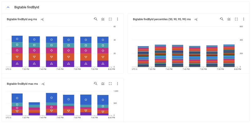
The application makes use of Spring Repositories for all persistence layer communication, which makes it very easy to set up the timing. We were able to set up auto-timing for all Repository methods. Out of the box, by enabling auto-timing you get the max, and the necessary metrics to calculate average. We additionally configured the application to gather percentiles metrics at 0.5, 0.9, 0.95, and 0.99. Auto-timing the repository methods also made it inconsequential where the API requests were coming from when running tests.
Running the Tests
The tests were conducted by running Locust in a Docker container on a laptop (or multiple containers when testing multiple regions). Locust is a pretty simple tool you can use for stress testing an application, or just for automating a bunch of API calls. We configured static IPs for each GKE cluster which allowed us to control which region we were sending traffic to. We used managed prometheus to get the metrics into Metrics Explorer, and created dashboards for the various databases.
Putting It All Together
We accumulated the data for each test into charts. For example:
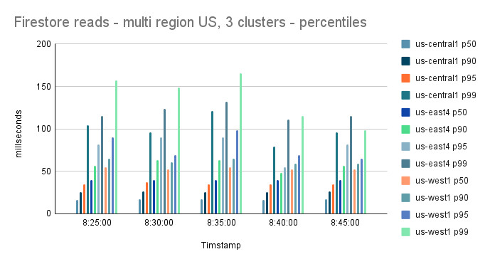
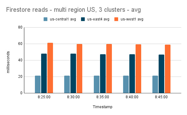

We then took the average of the averages for each test to give us some baseline latency numbers.


Drawing the Decision Tree
With the latency data gathered, we were finally able to draw the decision trees!
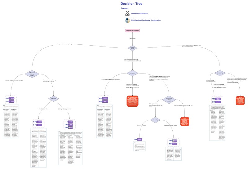
What helped us to significantly reduce the size of the tree was to focus our efforts on what were the 2 prevailing patterns used by Storefront.
- Sharded pattern - essentially distributed reads/writes
- Distributed reads - essentially teams write from an admin interface or some internal tooling and that gets distributed out to all the regions to be read from
We are calling the main decision point the “Location Needs” and we also have a small set of branches for applications that truly need just a single region.
We have a few negative result leaves for needs that cannot be met by current options. For example, there is no option that provides distributed writes or strong trans regional consistency.
We also tried to include some cost considerations in the diagram. For example, Spanner does not appear as an option for applications that only need a single region. For a single region application that needs a super high write throughput, it would work, but it would be far more expensive than the options listed, and that is why it was omitted.
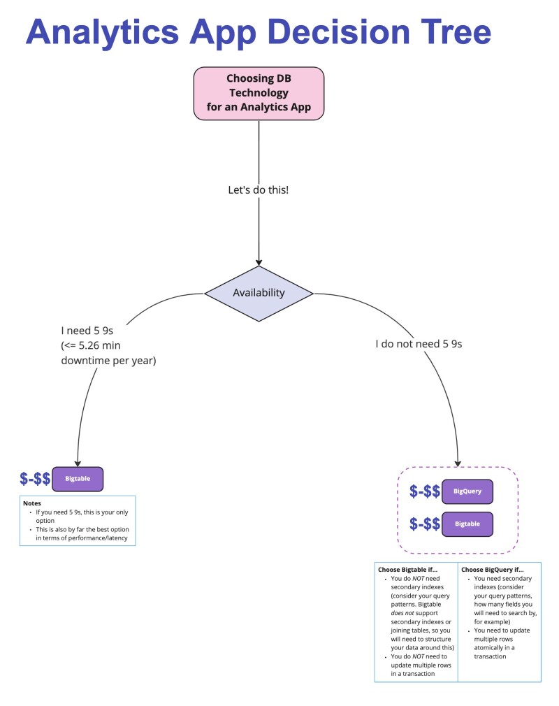
Where you see a table with multiple options, a notes section describes common features, and the split columns describe when to use one over the other.
Finally, we broke analytics concerns into a separate tree, because, quite frankly, BigQuery’s latency metrics do not make it a great choice otherwise. It is worth mentioning that using BigQuery with a JDBC driver and Spring Repositories is really not a good way to use it, and could certainly have contributed to the latency measurements.
Conclusion
It is not an easy task to create such a guide, and it will likely evolve over time. If we can use this guide to help our teams at least narrow down their choices, then it was well worth the effort.
