‘First impressions matter’.
While the above statement holds true for the very many aspects of life, it applies to E-commerce platforms as well.
Be it an accent chair designed for a neomodern apartment in Manhattan, New York or a double-hanging hammock styled for the patio facing a lush green backyard of a traditional farmhouse in Ozark, Arkansas - right from the conception of a product to its modeling to its manufacturing and finally its sale - the one question that remains common throughout the process for almost any type of a product is - Will it belong?
We work hard at Wayfair helping consumers feel confident items will fit into their homes. Part of our approach involves constantly innovating our process of selecting the best representations for our products, a process called Lead Image Selection. Since we want our visitors to be presented with the best representation of the product they want to buy, a very simple way of doing that is to predict for each image if it is ‘worthy’ of being the lead image. A study conducted by fellow data scientists concluded that images of products taken from a frontal angle generate higher Click-Through Rates (CTRs) than images showing back of the product. Being able to identify shot angles at scale, across the millions of items in our catalogue, is therefore important for identifying candidate lead images.

It’s common for vendors on E-commerce platforms these days to use images created from 3D models of products rather than actual product photographs. These 3D models are created from seed images which are in turn created by artists during the design processes. So, understanding shot angle also helps us identify whether we can build better 3D models of products, which also helps our customers get a better feel for products so that they feel confident in their purchases. An important component of being able to generate great 3D models is having seed images from enough angles, such that the whole SKU is covered. The process of checking if enough angles are being covered by a sample set of images is painstakingly lengthy and manual. Shot angle prediction along with a business layer logic (shown below) has increased automation for the visual vetting process.
https://storage.googleapis.com/wf-blogs-engineering-media/2020/07/61cc621e-image-1.png
What is shot angle?
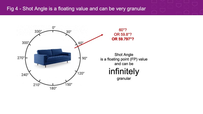
Simply put, shot angle is the angle between the face of a product and a (virtual) camera taking that image. In other words, it’s the angle that a product faces in the image.

Modeling approach for Shot Angle Prediction
While there are several simpler computer vision methods available for angle estimation for relatively homogeneous datasets - like pose estimation for humans, predicting angles for a diverse dataset like furniture is rather tricky and requires deep learning along with computer vision.

However, while deep learning models are good at classification, i.e. telling a cat from a dog or an apple from an orange, the angle is a continuous quantity.
Furthermore, telling a front-view of a sofa from a back one is more difficult than telling a cat from a dog, because of the similarity of features. One must also pay heed to the efforts that will go into quality assurance—it would be extremely tedious to have a human-in-the-loop setup for QA for a regression model, as it would require a human annotator to tag granular values for angle. We present below a comparison of the advantages vs. disadvantages of a pure regression vs. classification approach below.
Comparison of Modelling Approaches: Regression vs Classification
| Evaluation Criteria | Regression: Continuous Angle Values “Informative” | Classification: Discrete n-Zone Angle Values “Practical” | Reason for rating |
| QA Efforts | ✖ | ✔ | Humans can interpret discrete angle zones rather easily Example, tagging an image as “Front” is more easily recognized than tagging an image with 40° |
| Modeling Efforts | ✖ | ✔ | Classification requires fewer data points |
| Performance | ✔ | ✖ | It was observed that predictions have a lower categorical error when trained for regression than classification |
| Compatibility | Angle ⇔ Zone | No backward mapping Zone ⇏ Angle | Loss of information in moving from more to less granular structure |
| Overall | Classification is overall easier to work with but, Regression offers a very distinct advantage in terms of performance and compatibility | ||
Following a Hybrid Approach: Classification + Regression
Given the limitations of both a pure classification and a pure regression approach, we decided to combine methods in a hybrid approach.
Before we get into discussing how to create a hybrid network, it is important to address how to create a process that ensures optimal quality of the model. To this day, deep learning models are reliant on human annotated data. With seemingly varying levels of perceptions among human annotators, how do we create a dataset consisting of angle labels which are agreeable for if not all, then at least most of the annotators?
Generating labels for QA - A study on Human Perception and Rotated Objects
As QA is easier with zone labels, our goal was to divide 360° continuous angles into zones to form “Angle Classes”. To do this, we conducted an initial survey that showed there are 8 angle zones: Going around the circle in a clockwise fashion, we get Front, Front-right, Right, Back-Right, Back, Back-left, Left and Front-left. But how do we map angles to zones? In other words, how do we draw boundaries between various angle zones? At what angle does “Right” become “Front-Right”?

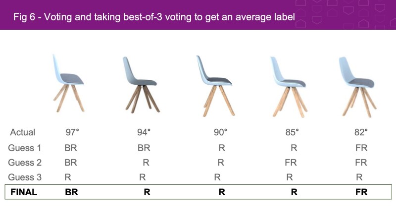
It’s fair to assume that various people would have different opinions about the “front”-ness or “back”-ness for an image. For example, in the image provided below, what person 1 can tell as “Front” may be “Front-Right” for person 2. So to generate labels for our training data, we synthetically generated 100 seed or reference images for the determined 8 angle zones using 3DSMax. Following that, we served 10,000 images to human annotators and asked them to select what angle zone suits best to the image. To avoid biases, annotators were not provided the exact degree values. Each image was labeled by 3 annotators. If a certain value received 2 or more votes, we assigned the label that value. In case a certain image garnered no agreement, we ignored it since such outliers only formed 6.3% of the dataset.

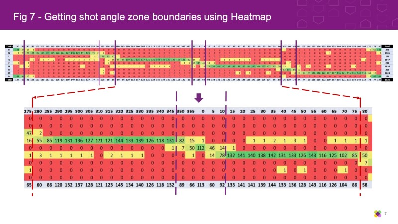
After this, we collected all the tags and compared them to the actual numerical values of the angles associated with the images. After generating a heatmap of angle zone tags against the actual numerical values of angles, the boundaries between angle zones emerged. For example, while going from 0° to 360° clockwise, around 15° “Front” starts appearing as “Front-Right”.

The study on human perception led to the following shot angle zone chart.


Representative images are shown along the angle zones to showcase how perception changes with rotation.
Accounting for different geometries

Shot angle labeling is not a one-size-fits-all approach. There is a huge difference in the geometries of various products. Some products are seemingly asymmetric in nature, like chairs and beds, meaning, they have a definite front. Others, like Wall Art or Area Rugs, have a planar geometry, and still others, like tables, are symmetrical, i.e. front and back look almost the same.
We, therefore, grouped the various product classes based on their geometries into the following categories:
- 3D Asymmetric: Objects that have a definite “Front”, for example, chairs, sofas, beds, etc.
- 3D Symmetric: Objects that look similar from “Front” and “Back”, for example, tables, desks, etc.
- 2D: Objects that are planar in structure, for example, wall art, rugs, curtains, picture frames, etc.
Note: We can’t define a shot angle zone chart for Round/Tripod/Triangular objects or objects that are symmetrical in 2 or more dimensions such that they look similar from all or many directions—in other words, objects for which one cannot define a “Front” or “Back” or “Left” or “Right” cannot have a zone chart.
Creating a ‘Hybrid’ Deep Learning Model
Since 2012, several deep learning models have been introduced to the Data Science community. We started experimenting with VGG16 as it is the easiest to understand and modified it to suit our purpose.
Bridging classification and regression
We implemented the hybrid approach in two steps:
- Pre-processing (Input) - We assign a numerical (or floating-point) value, i.e. canonical angle, to every zone. Canonical angle is simply the mid-point of the range covered by a zone. For example, the “Front-Right” zone covers angles from 15° to 75°. So, the canonical angle for this zone is 45°. Canonical angles for all the zones are listed in the “Zone Mappings” table above. For each training image, we simply replace the zone tags - i.e. F, FR, R, BR, B, BL, L, FL - by the canonical angles corresponding to the zones - i.e. 0°, 45°, 90°, 135°, 180°, 225°, 270°, 315°.
- Post-processing (Output) - Once the model predicts an angle (floating-point value), we then assign a zone label according to the range the output falls into. This way we are converting the result of the regression model to something that can be used for QA (for example, if the model outputs 52°, we assign the zone “Front-Right” to it since it lies in the range 15° - 75°).
Custom loss function - Calculating ‘Circular’ loss
Behind every successful deep learning model, there is an equally simple loss function. What loss function is to a Deep Learning model is like what a teacher is to a student. Our model needs to learn the concept of circularity, meaning, it needs to learn that both 0° and 360° are the same.
In theory, there are several versions of circular loss available in the art. We have defined a custom loss function using the Mean Square Error (MSE) or square of differences as follows:
loss = MSE(cos label) + MSE(sin label) = (cos θ - predicted cos)2 + (sin θ - predicted sin)2
We used MSE since it is a go-to concept for defining loss functions for regression-based models. In other words, MSE handles the regression part of our hybrid model. The θ above is discrete in nature, as described in the pre-processing step above. This makes for the ‘classification’ nature of the model.
Evaluating Model’s Performance during Training
When it comes to judging our model's performance, we calculate Zone-level accuracy.
Here, we check the model's performance against human-annotated data created using best-of-3 analysis mentioned previously. Our model predicts a numerical (floating point) value of the angle for an image. We consider a predicted angle (denoted by θ’) to be correct only if it lies in the correct zone identified during the annotation process.
For calculating accuracy, we need the predicted angle. At any point in time, we can retrieve the predicted angle (θ’) by the following relation:
θ’ = arctan2(predicted sin, predicted cos)
Once we have our θ’, we simply check what zone this θ’ belongs to and compare this predicted zone with the actual zone marked by humans. We repeat step this for all the images in our validation dataset and calculate the average zone accuracy (%) by this simple relationship:
Avg. Zone Accuracy = (Number of correct predictions / Number of Total Prediction) * 100
For math nerds
An interesting mathematical thing to note here is that when the model starts making correct predictions during its training phase, i.e. when predictions start getting closer to actual values, or angle θ’ ≈ actual angle θ, then our custom loss function degenerates to:
loss = 4 * sin2 ( (θ-θ’) / 2 )
Applying the small-angle approximation, we get
loss = (θ-θ’)2 ≈ MSE(θ’)
This may raise a question of why not training the model with loss function defined by MSE(θ’) itself in place of MSE(cos label) + MSE(sin label). We did not strictly compare the performance but an initial experiment revealed a very slow convergence during training when we used MSE(θ’) as the loss function. Maybe this question can be answered by having more experiments. But for the time, we stick with the loss function defined using trigonometric ratios.
Model Architecture

We created a quasi-VGG network that predicts a numerical value of the angle that takes 3 inputs: image along with sine and cosine values of shot angle.
Training Model with Synthetic Data
Ideally, it would be great for our angle prediction model to learn all the possible views of a product. That means teaching our model how the “front” zone could look like by giving it enough samples and the same process be repeated for all the defined zones. Again, ideally speaking, following the logic above, we are looking for a dataset that has images of many products marked for every degree of horizontal rotation. However, in the real world, very few datasets would provide such granular views of furniture products.
Hence, we turn to synthetic data. There are three key reasons behind using synthetic data:
- Our homegrown synthetic data generation process creates imagery that is reasonably close to what we get from vendors. So the chances of taking a performance hit due to domain gap are lower as the model would learn from images that are similar to what it will work during inference and production
- It allows us to train a model with images with granular angle information—instead of training models with only 8 numerical angle values, we can now train the model having a full 360° coverage.
- It addresses data imbalance in real-world images (i.e., most images belong to frontal zones): Training a model with imbalanced data weakens performance. A model trained with a dataset having a majority of “Front” images will result in poor performance on other zones like, “Back” or “Left”. We need a model that performs uniformly well on images from all possible angles. Even though data augmentation is available for striking a balance, it won’t provide enough variance.
Creating synthetic data with 3D Models
We utilized the 3D models for chairs and sofas from Wayfair’s 3D model’s repository and 3DSMax to create a dataset of training images. For each 3D model, we generated 100 views, i.e. 100 images, along with granular angle information. Below is a snapshot of this data set:

|
Creating environment images
The process described above-generated silhouette images or images of products with white background. For creating images of products in a typical home setting or environment images, we remove the white backgrounds of silhouette images and replace them with an environment.
Simply put,Environment image = Silhouette image - White background + Random environment
https://storage.googleapis.com/wf-blogs-engineering-media/2020/07/7990b20c-slide14.jpegResults
We performed inference on 2 sets of product classes on real-world silhouette images
- Chairs and sofas (520,000 images): We tested the model with 34 different classes of chairs and sofas
- Beds (97,000 images): We tested model with 12 different classes of beds
And here are our findings:
- We measure a zone-level accuracy - We consider a prediction by the model as correct only if the predicted angle lies in the correct zone identified during the best-of-3 human annotation process
- Overall accuracy for chairs and sofas was found to be 75% and which is quite comparable and almost at par with state-of-the-art accuracy as reported by this publication here.
- We perceive a lower accuracy of 66% for the beds dataset.
The above results are in line with our expectations since we created the shot angle zone chart and definitions using only the images from chairs and sofas. Applying the same definitions towards beds results in poor performance. This certainly provides some level of credence to the theory we proposed earlier that products with different geometries are perceived differently. For example, it may happen that while the “Front-Right” zone for chairs lies between 15°-75°, the same for beds could be a bit different.
Also, bridging the domain gap is tricky. While the process we followed during synthetic image creation helped us create a training dataset, which very closely resembled the images used by vendors and thus resulted in a strong baseline model, it’s not foolproof. Additionally, addressing the domain gap is a process with diminishing returns.

| 
|
Future Work
We are never done. The following are the identified areas where we can test our model and work towards making a more holistic algorithm:
- Environment images: Training the model with more environment images
- Conduct more human perception studies: Find a shot angle zone chart and set of zone definitions suited to each category of products. While this looks promising at first, this process, however could be affected by the law diminishing returns, especially for classes of products that fetch lesser revenue or have fewer than the others. Only more experiments will complete the whole picture. So a better approach could be to group as many similar looking products as possible and create shot angle zone definitions accordingly.
- Domain Gap Management: Use pre-processing methods like histogram matching on synthetic images to make them even closer to real-world images that we from from vendors
- Creating datasets, training and checking model's performance on product images belonging to other geometries like 3D Symmetric and 2D defined above.
References
ShapeNet
Designing Deep Convolutional Neural Networks for Continuous Object Orientation Estimation
https://arxiv.org/pdf/1702.01499.pdf
Pediatric Bone Age Assessment Using Deep Convolutional Neural Networks: https://www.researchgate.net/publication/321823302_Pediatric_Bone_Age_Assessment_Using_Deep_Convolutional_Neural_Networks3D Pose Regression Using Convolutional Neural Networks (Mahendran et al., 2017)
https://arxiv.org/abs/1708.05628
Geometric Loss Functions for Camera Pose Regression With Deep Learning (Kendall et al., CVPR 2017)
https://www.youtube.com/watch?v=Rp2Znu1ZJVA
https://arxiv.org/abs/1704.00390
Fast Single Shot Detection and Pose Estimation
https://ieeexplore.ieee.org/document/7785144
Exemplar part-based 2D-3D alignment using a large dataset of CAD models (Aubry et al., 2014)
Beyond PASCAL - A Benchmark for 3D Object Detection in the wild
http://cvgl.stanford.edu/projects/pascal3d.html
3D Models + Learning: Parsing IKEA Objects - Fine Pose Estimation (JJ Lim, 2013)
http://people.csail.mit.edu/lim/paper/lpt_iccv2013.pdf
3D Pose Estimation and 3D Model Retrieval for Objects in the wild (CVPR 2018)
http://openaccess.thecvf.com/content_cvpr_2018/html/Grabner_3D_Pose_Estimation_CVPR_2018_paper.html
Synthetic Viewpoint Prediction
https://ieeexplore.ieee.org/document/7801548
Geometric Deep Learning for Pose Estimation
https://ieeexplore.ieee.org/document/5995327

